

Most explanations of why steganography gets detected are theoretical. They describe a mechanism, work through why it leaves a trace, and leave you to assume that real tools actually look like the example.
This one isn’t theoretical. I read the embedding code of a small, publicly available open-source steganography tool — the actual source, not the README — and it makes nearly every mistake it’s possible to make, in one place. I’m not naming it or linking it. It’s an honest project by someone learning the field, the findings are about the code rather than the person, and a takedown by name would be neither fair nor useful.
There are three mistakes. The worst one doesn’t need statistical analysis to catch. It doesn’t need the password either.
First, What It Got Right
The encryption is genuinely well done, and that’s worth saying plainly before anything else.
The payload is encrypted with AES-256-GCM — an authenticated cipher, so a modified ciphertext is rejected rather than quietly decrypting into garbage. The salt is random per file, and so is the nonce. Nonce reuse and a hardcoded salt are two of the most common ways an otherwise reasonable implementation gets broken, and neither mistake is here.
So the content is protected. Extracting the payload bits without the password gets you nothing usable. That part of the job is done properly, and everything that follows should be read against it — this is not a story about someone who didn’t know what they were doing.
Mistake 1: The Placement Is Completely Predictable
The payload goes into the image in raster order. Top-left pixel first, then the next, then the next, one bit into each colour channel, until the payload runs out.
Every file. Every time. The placement doesn’t depend on the password, and it doesn’t depend on the image.
That costs three separate things.
There is nothing to search. An analyst doesn’t have to work out where the data might be. The first pixel is the first pixel.
The disturbance is concentrated instead of spread. The payload occupies a contiguous block at the top of the image and nothing below it. A statistical test that might read as marginal across a whole image reads as unambiguous when it’s run over the region that actually carries data — because within that region, effectively every available bit has been written to.
It’s blind to the picture. A flat expanse of sky and a patch of dense foliage get treated identically, when they are not remotely equivalent places to put a modified bit. A clean gradient shows a single altered bit; a busy, textured scene can absorb far more before anyone would notice — which is the whole reason steganography is possible at all. I went into this at length in where the data actually goes. A tool that writes in raster order isn’t making that distinction, because it never looks at the picture in the first place.
Mistake 2: LSB Replacement
The write primitive is least significant bit replacement: take the bottom bit of a colour value and overwrite it with a payload bit.
I covered this one in depth a few weeks ago. LSB replacement leaves three separate statistical signals — a comb pattern in pixel value pair histograms, a shift in bit-plane randomness, and a broken correlation that real camera noise doesn’t break — and RS analysis turns those into a quantitative test that estimates the embedding rate rather than just answering yes or no. I won’t repeat the mechanics here.
What’s worth adding is how badly this compounds with mistake 1. RS analysis reports asymmetry in proportion to how much of the region you tested was modified. Run it across an entire image with a small payload hidden in the first few rows and the signal is diluted by all the untouched pixels. Run it over just those first few rows — which mistake 1 tells you exactly how to find — and the embedding rate in that window is close to saturation. That’s the loudest possible reading for a test that measures exactly this.
The two mistakes aren’t additive. The first one makes the second one easy.
Mistake 3: A Plaintext Length Header, Always in the Same Place
This is the one that matters, and it needs no statistics at all.
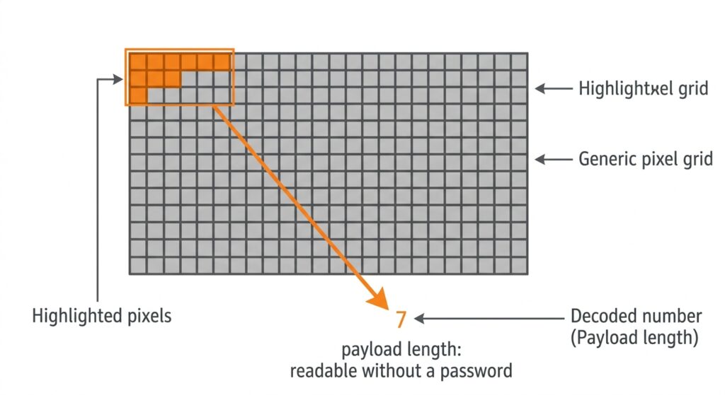
Before any encrypted payload goes into the image, the tool writes a four-byte value recording how many bytes follow. That header is not encrypted. It is not keyed. It does not move. It sits at the very start of the embedding sequence, in the clear, in every file the tool has ever produced.
Read those bits from the offset you already know, and interpret them as an integer.
In an untouched photograph, those low-order bits are whatever the sensor noise happened to leave behind, so the number you get back is arbitrary — anywhere across a four-billion-value range. In a file this tool produced, the number is the real payload length: small, plausible, and comfortably smaller than the image could hold.
One number, two answers. A value in a sane range says something is hidden here. The value itself says how much.
No password. No brute force. No chi-square test, no RS analysis, no statistical modelling of anything. Just knowing where to look and reading the number back.
And it doesn’t stop at detection — the length tells you precisely which pixels carry the payload and where it ends, which sharpens every statistical test you might run afterwards. The header hands over both the presence and the map.
The Lesson: Content and Presence Are Separate Guarantees
The three failures here are independent problems, and that’s the part worth carrying away.
Predictable placement is a search problem. A detectable write primitive is a statistics problem. Metadata in the clear is a format problem. Fixing any one of them does nothing for the other two. You can fix placement and still be caught by the histogram. You can fix the histogram and still be caught by the header.
And strong encryption — which this tool genuinely has — doesn’t touch any of the three, because it was never solving that problem. Encryption answers “can you read what’s inside”. Steganography has to answer “can you tell there’s anything inside”. Those are different questions — two separate layers, not one feature — and a tool can answer the first perfectly while failing the second to anybody who knows the format.
That distinction is not academic. For most people who reach for steganography rather than plain encryption, the thing they were trying to avoid was the question — and the question gets asked the moment presence is established, no matter how good the cipher is.
And this isn’t the beginner’s error it might look like from a distance. Getting authenticated encryption right — correctly salted, correctly nonced, tamper-evident — is the part most implementations fumble, and this one didn’t. A length written in the clear is precisely the kind of detail that survives review, because it sits just outside the part everyone thinks to check. That’s what makes it worth naming rather than laughing at: this failure mode catches tools that got the hard part right.
Checking What a File Actually Gives Away
A hidden payload is only one of the things a file gives away without being asked. Its structure, its metadata, its compression fingerprint and its noise statistics all say something, and I’ve mapped the full set of them in the complete guide to JPEG forensic analysis.
If you want to know what one specific image discloses, that’s what snapWONDERS forensic analysis is for. No account required.
The cipher protects what’s inside. The format is what gives it away — and the format is the part nobody re-reads.
Kenneth Springer is the founder of snapWONDERS, a digital forensic analysis platform for images and video, and built snapWONDERS Vaultify, its steganography platform. He works on both sides of this problem — the statistical tests that catch hidden data and the engineering of hiding it well — which is why an audit like this one reads as a checklist rather than a curiosity. snapWONDERS forensic analysis — no account required.